NZ Macroconomics — I
Published on
Contents
A new series on some aspects of NZ macroeconomics. Topics are just whatever I bother to look at and write-up. Today, the Real NZ government surplus(deficit).
NZ Government Real Deficit
This is topical whenever there is a significant inflation event, and such has occurred post-COVID.
We need a formula that can show how a nominal deficit can become a real surplus from the non-government sector’s perspective when inflation is high enough.
The question is about how inflation affects the real value of government debt. Inflation can can turn a nominal deficit into a real surplus! That’s bad for an economy with a growing population.
The basic formula would be:
$$
\text{RealDeficit}_n = \text{NominalDeficit}n - (\text{InflationRate}\times \text{GovDebt}{n-1})
$$
For example, if:
(i) Nominal deficit = $1 trillion
(ii) Outstanding debt last year = $30 trillion
(iii) Inflation = 5%
then,
$$
\text{Real deficit} = 1T - (0.05 \times 30T) = 1T - 1.5T = -0.5T
$$
This would actually be a real surplus of 500 billion, despite the
nominal deficit. Which would be very bad if the population was
growing, which it is in Aotearoa. We are likely to see more unemployment,
not less.
For hardline MMT: the price level is irrelevant, full employment is the goal & a lowest real wage rising the fastest of all wages.
Why are we using the government debt as the adjuster?
Let’s think this through:
- A nominal deficit of $1T means the government is injecting 1T of purchasing power into the non-government sector.
- At the same time, inflation (say 5%) is reducing the real value of all nominal assets held by the non-government sector, including government securities (the $30T).
The original formula actually does capture this correctly I beleive: Real deficit = Nominal deficit - (Inflation Rate × Outstanding Debt).
This works because: (i) The nominal deficit represents new purchasing power injected (ii) (Inflation Rate × Outstanding Debt) represents the loss of real purchasing power on existing government securities held by the non-government sector.
This negative value (real surplus) means the non-government sector is actually losing purchasing power in real terms, despite the nominal deficit, because inflation’s erosion of the value of their government asset holdings exceeds the new purchasing power injection.
Population Growth
If we were going to be real meta-nerds, we should make a population size adjustment, since if the population shrunk then a nominal government surplus might still be a real deficit spending!
Here is the python for that:
pop_growth_rate = df['Population'].pct_change()
real_deficit_adjusted = df['GovExp'] - df['GovRev'] - (inflation_rate - pop_growth_rate) * df['NZ_GDEBT']
I don’t know about you, but I prefer the mathematics straight, so it would be:
$$ \begin{align*} g_p &= \frac{P_n - P_{n-1}}{P_{n-1}}, \\ \text{RealDeficit}_\text{adj} &= \text{NominalDeficit} - (\pi - g_p)\cdot \text{GovDebt} \end{align*} $$
where actual inflation rate $\pi$ is, $$ \pi = \frac{\text{CPI}_n - \text{CPI}_{n-1}}{\text{CPI}_{n-1}}. $$
Note: You would have to apply the ratio $\pi$ there for the CPI if it
was the Index value (100 – 1000) or whatever. But our FRED series we
use CPGRLE01NZQ659N is the percentage change, so we are ok. I call
it “CPI” sometimes in my python dataframes, but I shouldn’t, it really
is the backwards looking rate of inflation proxy! That means it is
also not today’s rate of inflation!
Avoid Confusion with Real Goods Deficit Spend
The spending power of the government deficit spending alone is a different sort of “real deficit”. It is merely the inflation adjusted raw deficit spending. You would compute it via, $$ Deficit_\text{adjusted} = \text{NominalDeficit} \cdot \frac{\pi_{n-1}}{I\pi_n} $$ where $n$ is the year, so $\pi_{n-1}$ is the inflation rate for the previous year.
This Deficit is always going to have the same $\pm$ sign as the Nominal Deficit, so does not reflect the real terms of the add from government deficit spending. (Obviously, since the outstanding net currency = total GovDebt is not in the formula anywhere.)
Bank Credit
Bank credit does not add any net currency assets into the economy, but it can boost circulation of the currency if the private household debt level is not too high. One should probably factor this into the overall Real Deficit of the whole economy, but I am not going to fetch all the NZ banking data, so I will leave that to PhD students.
We want to spank the government for being naughty, not private households.
Back-of-the-envelop Real Deficit(Surplus)
NZ Treasury statement 2023 was:
- Net GovDebt = 18% of GDP.
- GDP = 2.52175506110 USD. NZ-Tsy nominal GDP = 3.95896 NZD.
- Expenditure (core)= 1,276 billion nzd.
- Revenue (core) = 1.124 billion nzd.
- Expenditure total = 1.61822 billion.
- CPI inflation = 5.7% (average), mid-year was 5.3%.
GDP agrees with World Bank . To convert to NZD the effective exchange rate was 1.5699 nzd per usd. Looks about right, daily was around 1.55 to 1.75.
So Net GovDebt = $3.95896\times 0.18$ $= 0.7126$ billion nzd. FRED
series NZLGGXWDGG01GDPPT has GrossGovDebt = 31.35% of GDP = $1.247$ billion nzd.
Nominal deficit = $1.276 - 1.124 = 0.152$ billion nzd.
Plugging this in: $$ \text{Real deficit} = 0.152 - 0.057\times 1.247 = 0.081 \,\, \text{bil. nzd} $$
To validate with external data like FRED and OECD, today, at the time of writing we can look at the 2021, 2022 , 2023 Treasury Statements as a representative sample.
The closet FRED series is NZLGGXWDGG01GDPPT and is in units %GDP, so we
need to pull the NZ GDP numbers as well, MKTGDPNZA646NWDB. FRED has these
in USD, so we have to pull the currency conversion CCUSMA02NZM618N series too. Unfortunately this FRED NZ GovDebt series only goes back to 2016. So we are
only using the FRED for data validation. The clunky
NZ Treasury spreadsheets
will have to be out painful data source for more historical analysis. More
on that next chapter! It was a real mission to get those look-ups automated.
NZ Treasury spreadsheets report fiscal year-end, so June. But we can use the December Monthly statements for the calendar year.
I eventually got too tired of extracting the spreadsheet data. So I used some series from the FRED and the OECD portal to run numbers for the limited range allowed, 20126–2022.
Real Deficit Results (2016–2022)
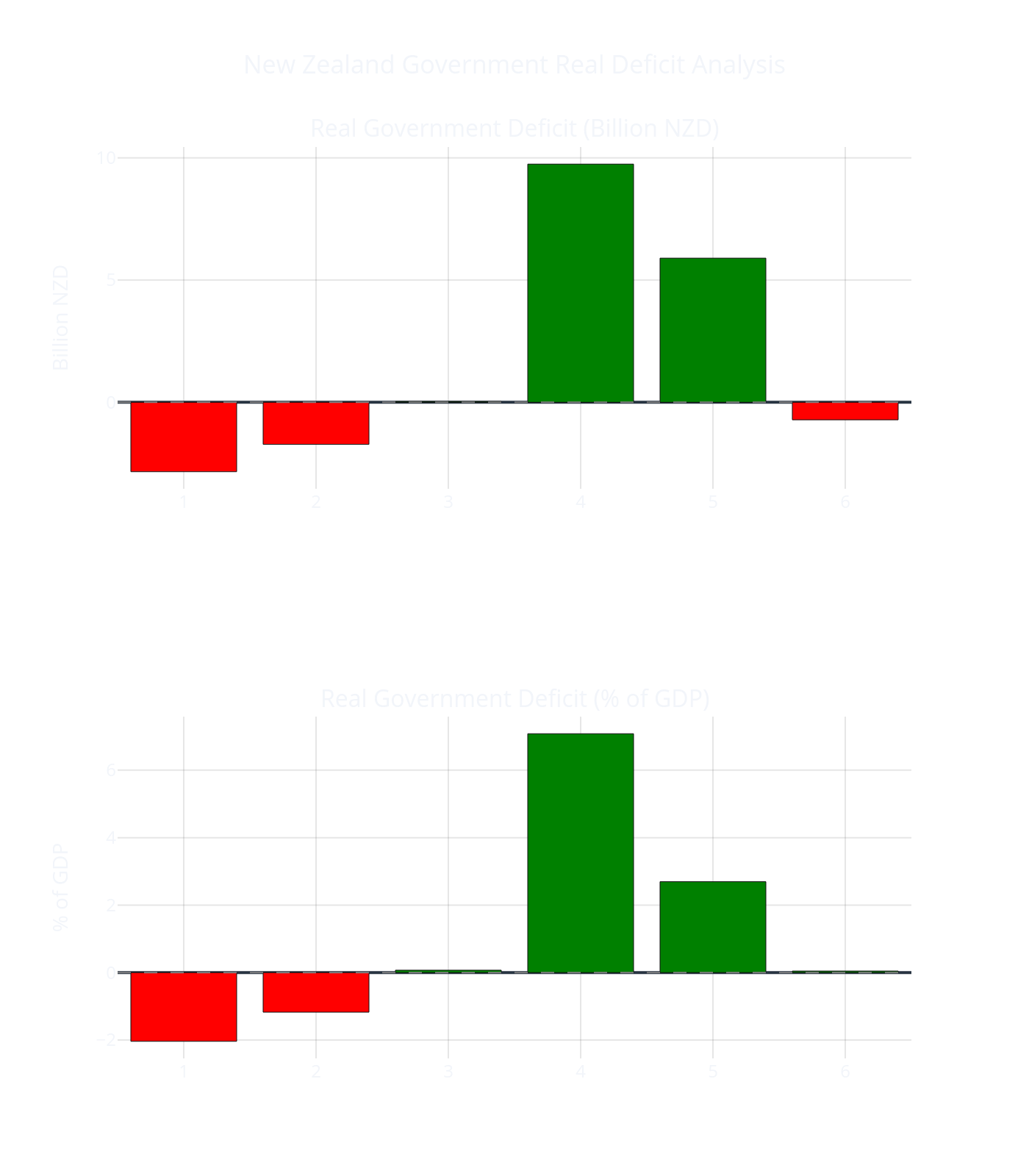
Need it be said? Green bars + are government deficit = non-government savings. Green is good. Or, +deficit of someone else ifs good for us, it is our +saving.
The rest of this chapter is technical mumblings and fumblings — just a crude journal on how I was struggling to get consistent data sources.
Sample Raw NZ Tsy Figures
A few series are reported as %GDP, so we need to square the GDP numbers. The first GDP column is direct from NZ Treasury Statements. Some years GDP is not easy to find reported in nominal nzd in the Treasury Statement, so in those case I estimate from other figures given twice, once as %GDP.
For exchange rate, (cur) means the Dec. of the last year of the FRED GDP data, which was 2023. I am not sure if this is the correct adjustment to the FRED GDP.
| Year | GDP (nzd_bil) | fred_gdp (usd) | usd:nzd | fred_GDP (nzd) |
|---|---|---|---|---|
| 2021 | 343.36 | 253.64 | 1.41 (ave) | 358.6 |
| 2021 | '' | '' | 1.39 (jan) | 352.6 |
| 2021 | '' | '' | 1.47 (dec) | 372.8 |
| 2021 | '' | '' | 1.60 (cur) | 405.8 |
| 2022 | 359.476 | 246.73 | 1.578 (ave) | 389.3 |
| 2022 | '' | '' | 1.575 (dec) | 388.6 |
| 2022 | '' | '' | 1.60 (cur) | 394.8 |
| 2023 (a) | 419.810 | 252.17 | 1.56 (ave) | 394.3 |
| '' | '' | 1.60 (dec) | 403.472 | |
| '' | '' | 1.60 (cur) | 403.472 | |
| 2023 (b) | 400.818 |
The discrepancies could be due to NZ Tsy using July-to-June as the “year” (fiscal year).
The World Bank values the FRED uses are calendar year. See World Bank Helpdesk .
FRED seems consistently on the high side of NZ Tsy, maybe they do NIPA accounting differently? Also, the source for the FRED series is the World Bank. The source data uses “current USD” — but I find it hard to know what that means, what date is “current”. The metadata says the WB uses “single year official exchange rate”. They have a page for that here Official LCU exchange to USD which for “current” being 2023 was 1.63. But you see from the table that does not improve the agreement with NZ Tsy nominal GDP figures, which are not price adjusted.
We might be ok using the FRED data with a calibration. For that we want to look at NZ Tsy Deficits and GovDebt and compare with OECD. Working with the NZ Tsy Statements was a mess without some automation, since the figures published are monthly, or to-June fiscal year.
| Year | GovExp (bil. nzd) | GovRev (bil. nzd) | GDP (bl. nzd) |
|---|---|---|---|
| 2021 | 197.70 (total) | 189.466 (total) | 343.36 |
| '' | - | 142.343 (tax) | '' |
| '' | - | 152.791 (crown) | '' |
| 2022 | 225.225 (total) | 207.819 (total) | 359.476 |
| '' | - | 158.551 (tax) | '' |
| '' | - | 171.621 (crown) | '' |
To compare NZ Tsy with OECD data (via World Bank I think) we need to convert to %GDP:
| Year | GovExp (%gdp) | OECD GovExp (%gdp) | GovRev (%gdp) | OECD GovRev (%gdp) |
|---|---|---|---|---|
| 2021 | 57.58 (total) | 44.9 | 55.18 (total) | 40.78 |
| '' | - | 41.46 (tax) | - | |
| '' | - | 44.498 (crown) | - | |
| 2022 | 62.65 (total) | 42.52 | 57.81 (total) | 40.88 |
| '' | - | 44.11 (tax) | - | |
| '' | - | 47.74 (crown) | - |
Interim Status: We only get $\pm$ 10 to 30 million NZD missing here and there? Good enough? I do not mind that the percentage deficits are lower for the Tsy data then for the OECD.
The more important series to check are GovDebt, GovExp, GovRev. The change in GovDebt needs to be consistent with (GovRev$-$GovExp). But I will get the better quality NZ Treasury data in the future, time permitting, then e-run the RealDeficit analysis.
Lesson: You never want to run serious econometric analyses with nominal data. You want to convert to a dimensionless ratio.
For our Real Deficit analysis what can we do? We only need to make sure our NominalDeficit and GovDebt numbers are based on the same year/price. I think although using FRED is highly convenient, if we were being serious we would use the NZ Treasury Statements, because the RealDeficit calculation is only using one year of data, so price level adjustments will be irrelevant.
However, when reporting the RealDeficit it would be better to convert to dimensionless units, like %GDP for the given year. Then the whole RealDeficit time series will be year-relative and dimensionless.
The purpose of data needs to be born in mind. We are interested in how a Nominal GovDeficit can become a RealSurplus. That is a year-by-year matter. We would not be looking to use a value for RealDeficit in NZD from 1980 to say anything about 2024, since prices changed. But we could say something about the “health” of the NZ economy by comparing the RealDeficit as % annual nominal GDP from 1980 to 2024. So the above conclusion & lesson seems justified.
For GovDebt the FRED series NZLGGXWDGG01GDPPT is closest, but only
goes back to 2016. Until I get the awful spreadsheet automation work
sorted out for the NZ Treasury Statements, I will just use the FRED
series, so only report the RealDeficit from 2016–present.
I am lazy, so I will use the FRED where possible. For For this
purpose I think it is fine the use the following series:
| Measure | Source | Code | Units |
|---|---|---|---|
| GDP | FRED | MKTGDPNZA646NWDB | usd |
| $\pi$ (inflation) | FRED | CPGRLE01NZQ659N | - |
| GovDebt | FRED | NZLGGXWDGG01GDPPT | pct_gdp |
| USD2NZD | FRED | CCUSMA02NZM618N | - |
| GovExp | OECD portal | A.NZL.OTES13 | pct_gdp |
| GovRev | OECD portal | A.NZL.OTRS13 | pct_gdp |
In my python script real_deficit_data.py I only run the FRED fetch.
The OECD data was needed for other projects, and runs separately
saving to a CSV file. So in the RealDeficit script I just load that file.
We then output a RealDeficit CSV time series, and a nice plotly plot.
Pictures Tell the Story
While we are here, it is good to look at the OECD portal NZ GovRev and GovExp, the difference being a nominal deficit(surplus). Hopefully this lnk here, OECD NZ government deficit(surplus) will open in your browser. In case not I took a snapshot c.2024, which only ran from 1986 to 2023.
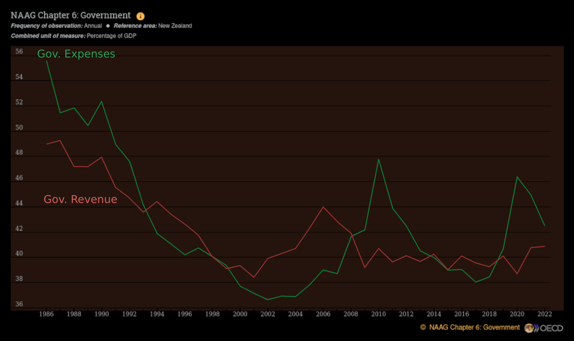
First, note tax revenues are the bulk of the Crown revenue. It would be nice to overlay the recession period shadows, as one does, but I did not bother, so apologies. However, you can see when the decline in percent GDP expenditures goes faster than decline in tax revenue it spells trouble.
When the red line is above the green = danger!
Also, the portrait on the NZ economy is dynamic, you can see tax revenues fall off over the financial crisis period from 2006 to 2010. Even before the crisis proper befell the USA and Europe, NZ was already going in a declining turn-over direction.
This speaks to Mosler’s Seventh deadly innocent fraud: higher government deficits today means higher tax returns tomorrow. The myth is that it is a bad thing, when in fact it si a good thing. The NZ government does not need to raise extra taxes when it deficit spends, the tax return will automatically reflux higher of the economy is doing well. The government may want to raise taxes in the future to cool off inflation, but it does not ave to do so.
Cooling off inflation is one use of taxation, but it is not the primary use, and is not even all that essential. The primary purpose of taxes (the liabilities that is, not the receipts) is to create a demand for the currency in the non-government sector.
Checking Flows
For GDP (a flow variable) if you grab monthly data and wish to convert to annual YE, then it is a good idea to check your down sampling preserves the sum.
Down Sampling
This is easy, pandas provides a resample() method. For a stock
variable we would use an average,
df.resample('YE').mean()
of course, that is coarse and ignores seasonality.
For a flow variable we can use:
df.resample('YE').sum()
Here is a quick copypasta snippet to use for testing:
# Generate dummy date monthly 2021, 2022, and 2023
date_range = pd.date_range(start='2021-01-01', end='2023-12-31', freq='ME')

# Generate random GDP values in billions
np.random.seed(0)
gdp_values = np.random.rand(len(date_range)) * 1000  # GDP values between 0 and 1000 billion

# Create the DataFrame
df = pd.DataFrame({'Date': date_range, 'GDP_bil': gdp_values})

# Set the 'Date' column as the index
df.set_index('Date', inplace=True)
To down-sample the flow variable:
gdp_annual = df.resample('YE').sum()
After this, the check the flow accumulation was preserved run:
>>> gdp_annual =  df.resample('YE').sum()
>>> gdp_annual
                GDP_bil
Date
2021-12-31  7478.282791
2022-12-31  7172.599144
2023-12-31  5482.526794

>>> gdp_monthly_sum_by_year = df.groupby(df.index.year).sum()
>>> gdp_monthly_sum_by_year
          GDP_bil
Date
2021  7478.282791
2022  7172.599144
2023  5482.526794
All good.
Up Sampling
Suppose we had Annual frequency data, and wanted Monthly. For a stock variable we can simply interpolate linearly (again ignoring seasonality). For a flow variable we can distribute at random, assuming a uniform distribution.
For Stock Variables:
df_monthly = df_annual.resample('ME').ffill().interpolate(method='linear')
For Flow Variables:
df_monthyl = df_annual.resample('ME').ffill() / 12
Here is a dummy example:
# Create a DataFrame with Annual Data for three years
data = {
    'Date': ['2021-12-31', '2022-12-31', '2023-12-31'],
    'GDP': [24000, 25000, 26000],  # Annual GDP in billions
    'GovDebt': [100000, 110000, 120000]  # Government Debt in billions
}

df_annual = pd.DataFrame(data)
df_annual['Date'] = pd.to_datetime(df_annual['Date'])
df_annual.set_index('Date', inplace=True)

# Display the annual DataFrame
print("Annual DataFrame:")
print(df_annual)

# Upsample to Monthly Frequency
df_monthly = df_annual.resample('ME').asfreq()

# Distribute Flow Variable (GDP) evenly across months
df_monthly['GDP'] = df_annual['GDP'].resample('ME').ffill() / 12

# Interpolate Stock Variable (GovDebt) linearly
df_monthly['GovDebt'] = df_annual['GovDebt'].resample('ME').ffill().interpolate(method='linear')

print(df_monthly)
To double check the stock:
>>> df_annual
              GDP  GovDebt
Date
2021-12-31  24000   100000
2022-12-31  25000   110000
2023-12-31  26000   120000

>>> debt_check = df_monthly['GovDebt'].resample('YE').last()
>>> debt_check
Date
2021-12-31    100000
2022-12-31    110000
2023-12-31    120000
Freq: YE-DEC, Name: GovDebt, dtype: int64
Good.
To double check the flow:
gdp_monthly_sum_by_year = df_monthly['GDP'].groupby(df.index.year).sum()
But this was “dumb”. It is more natural to impose a monthly fluctuation. Even though this will be fake, we are doing this pedagogically as a build-up. The “proper” way to up-sample would be to find some believe monthly correlator. Absent that sophistication, let’s just do it with a simple random fluctuation.
Adding Monthly Fluctuations
If we do not want to worry about seasonality correlation we can just assume uniform distributions, and add a random fluctuation. To be more nuanced and correlate the monthly fluctuations we could use some other data we think is correlated, like SPX, or monthly GovDeficit, or whatever econometric series is available at the higher frequency and which we believe might be correlated.
I have not gone to that bother in this write-up, so we’ll just look at a random uniform distribution. Here I use the yearly variance to infer a monthly variance.
import pandas as pd
import numpy as np


def upsample_flow_annual_to_month(df, column):
    """
    Upsample a flow variable (e.g., GDP) from annual to monthly frequency with random fluctuations.
    """
    # Create a date range for the monthly frequency
    monthly_dates = pd.date_range(start=df.index.min(), end=df.index.max(), freq='ME')
    monthly_df = pd.DataFrame(index=monthly_dates)
    # Repeat the annual values to create a monthly average
    repeated_annual_values = np.repeat(df[column].values, 12)[:len(monthly_dates)]
    # Calculate monthly variance based on annual variance
    annual_variance = df[column].var()
    monthly_variance = annual_variance / 12
    # Generate monthly fluctuations around the average
    np.random.seed(0)  # For reproducibility
    monthly_fluctuations = np.random.normal(loc=0, scale=np.sqrt(monthly_variance), size=len(monthly_dates))
    # Distribute the annual sum across months with fluctuations
    monthly_df[column] = repeated_annual_values / 12 + monthly_fluctuations
    # Renormalize to ensure the annual sum is preserved
    for year in df.index.year.unique():
        monthly_df_year = monthly_df[monthly_df.index.year == year]
        annual_total = df.loc[df.index.year == year, column].values[0]
        monthly_total = monthly_df_year[column].sum()
        normalization_factor = annual_total / monthly_total
        monthly_df.loc[monthly_df.index.year == year, column] *= normalization_factor
    return monthly_df


def upsample_stock_annual_to_month(df, column):
    """
    Upsample a stock variable (e.g., GovDebt) from annual to monthly frequency with linear interpolation.
    """
    monthly_df = df.resample('ME').asfreq()
    monthly_df[column] = df[column].resample('ME').ffill().interpolate(method='linear')

    # Renormalize to ensure the year-end stock value is preserved
    for year in df.index.year.unique():
        month_end = f'{year}-12-31'
        if month_end in monthly_df.index:
            monthly_df.loc[month_end, column] = df.loc[f'{year}-12-31', column]
    return monthly_df


def upsample(df, column, var_type='flow'):
    """
    Upsample a variable from annual to monthly frequency.

    Args:
    - df: Pandas DataFrame with annual data.
    - column: The column name to upsample.
    - var_type: Type of the variable ('flow' or 'stock').

    Returns:
    - A DataFrame with monthly frequency.
    """
    if var_type == 'flow':
        return upsample_flow_annual_to_month(df, column)
    else:
        return upsample_stock_annual_to_month(df, column)
Now we can run dummy data tests:
# Mock Up Dummy Example
# Create a DataFrame with Annual Data for three years
data = {
    'Date': ['2021-12-31', '2022-12-31', '2023-12-31'],
    'GDP': [24000, 25000, 26000],  # Annual GDP in billions
    'GovDebt': [100000, 110000, 120000]  # Government Debt in billions
}

df_annual = pd.DataFrame(data)
df_annual['Date'] = pd.to_datetime(df_annual['Date'])
df_annual.set_index('Date', inplace=True)

# Upsample GDP (flow variable)
df_monthly_gdp = upsample(df_annual[['GDP']], 'GDP', var_type='flow')

# Upsample GovDebt (stock variable)
df_monthly_govdebt = upsample(df_annual[['GovDebt']], 'GovDebt', var_type='stock')

# Combine the upsampled data
df_monthly = pd.concat([df_monthly_gdp, df_monthly_govdebt], axis=1)

# Display the monthly DataFrame
print("\nMonthly DataFrame with upsampled GDP and GovDebt:")
print(df_monthly)
Check the flow conservation law:
gdp_check = df_monthly['GDP'].resample('YE').sum()
Older Check
- GDP = 3.59476 billion nzd.
- Net GovDebt = 0.61829872 billion nzd or 17.2% of GDP.
- Gross GovDebt = 1.18986556 billion or 33.1% of GDP.
Check: From OECD and FRED:
- FRED
NZLGGXWDGG01GDPPT: GovDebt (total) 31.9% of GDP. - OECD: Gross GovDebt (total) 59.59% of GDP.
Unfortunately, the API for Treasury data is an excel spreadsheet 🤣.
But I am glad I checked, since it looks like I had been using the
wrong FRED series DEBTTLNZA188A instead of the series more in alignment
with NZ Treasury which is NZLGGXWDGG01GDPPT.
Given the way the GovDebt is published it is probably a good thing that what matters for MMT analysis is more the change in the GovDebt. Since the outstanding absolute debt is really just an already established price level effect, and we know the price level roughly from other data. Further, what matters is relative prices, price::wage ratio for necessary goods, and purchasing power, not the absolute price level.
Time Series Automation
I thought it worthwhile automating a time series for the Real Deficit. It might be published somewhere else, but repetition does not hurt.
The USA Case
For empirical data input we have:
- MTSDS133FMS - Monthly Treasury Statement (Federal Surplus or Deficit)
- PCEPI or CPI - Price indices for inflation adjustment.
- Outstanding Debt Effect: the real deficit/surplus calculation should account for how inflation erodes the real value of the existing . debt stock, not just the nominal deficit flow. We’ll need:
- Total outstanding government debt (we can use GFDEBTN from FRED).
The FRED series ID’s just given will let you run a USA analysis, but we are interested in the NZ analysis at Ōhanga Pai.
The NZ Case
I think we can fetch most stuff from the FRED, but if not the BIS portal is a good first fallback, then the OECD portal. The latter two are clunkier to navigate, but here are some tips.
First, you only need to do this once, since we will get python code for automating future data updates.
- Go to https://data.bis.org/
- In the search box type a short accurate description of the series you
want, .e.g
NZ government total debt. - Select from the result the series that looks like a closest match. For example, I selected https://data.bis.org/topics/LBS/BIS,WS_LBS_D_PUB,1.0/Q.S.C.D.TO1.A.5J.A.5A.G.NZ.N
- Up on the top right of the webpage, above the Bookmark button click the “Export” button,
- Click on the “Code Snippet” tab.
- Python radio button is default, so now just scroll down to the code snippet and copy using the copy button icon. Paste into your python script.
- Note the BIS units for this series are US$mil., so we do not need to convert (our other islm data series were converted to millions of usd.)
Others for CPI (proxy for Inflation) and the deficit(surplus) :
TODO
CPI?
Deficit?
The BIS are a bit of a pain, since the TIME_DATE column has
format yyyyy-Qn.
We want to convert Quarters into yyyy-mm-01 dates. The BIS docs suggests
the quarters are ending, so we want our actual datetimes to be end of
March, September and December, but offset one day to 1st of the next
month. So the quarters I use are e.g.,
2024-01-01
2024-04-01
2024-07-01
This function will do that for you:
def convert_quarter_to_date(quarter_str):
    period = pd.Period(quarter_str, freq='Q')
    start_of_next_quarter = period.asfreq('Q-JAN').start_time + pd.DateOffset(months=3)
    first_of_last_month = start_of_next_quarter - pd.DateOffset(months=1)
    return first_of_last_month
Problems
Problem 1.
An immediate problem was that the BIS data set I choose did not look
like the NZ government debt. It was some obscure banking composite. But
it might be close to the series we ultimately want. So I had a go at
using the OECD SDMX-JSON Rest-API.
Problem 2.
The OECD Gross GovDebt figures are ballpark 59% of GDP (2022), whereas
NZ Treasury quotes 33.1%.
The FRED series DEBTTLNZA188A is close to the OECD. No good!
The FRED series NZLGGXWDGG01GDPPT is closer to NZ Treasury, but
starts at 2016. SO is not so useful.
I think we should be using the NZ Treasury Statements. But they are excel spreadsheet files. I did automate some of that, so will return to look at making a cron job for updating the data. The main thing is not not mess with the historical data, and only do a most recent years update/append.
OECD API
The Expenditure and Revenue series from the OECD are useful for comparing with the NZ Treasury data pull. This is just for data validation. I prefer to use the NZ Treasury Statements as the main source.
The NZ Government Expenditure and Revenue series seem to be available, the difference of these two aught to be our $(G-T)$. Also a ‘Gross debt of general government’ series is published, the year-on-year change in that should be close tot $G-T)$. All these series are in units ‘% of GDP’, so we need to fetch the GDP data too.
In case I forget, here is the way to get this data.
- Go to the explorer https://data-explorer.oecd.org/
- Put in a search, “Government expenditure” should do the trick, or “National Accounts at a Glance (NAAG) Chapter 6: Government”. I actually got there from a higher level overview of the OECD statistics here: https://www.oecd.org/en/data/indicators/general-government-deficit.html?oecdcontrol-8478925713-var1=NZL .
- Deselect all the other countries in the Region filter, I left New Zealand and the USA, since I want to check the USA against the FRED as my initial data validation.
- We should be on the “NAAG Chapter 6: Government” page.
- In the Measure filter select what you want, I went for (1) Expenditure, (2) Revenue. (We do not want the “Gross debt” series since that confounds cross-border stuff and “all currencies”.)
- In the Time period filter select the max range (1970 to present).
- Click on the Chart header to check the plot is ok.
- Click on “Developer API” on the top right of the dashboard.
- Change “SDMX flavour:” to “Time series” option.
- Copy the supplied Data query URL.
Now we need to paste this URL into our python script and make the request.
Your python snippet or URL will have the present date hard-coded, so it is good to make a str replacement in your script for this, so that you do not have to change the code in the future.
After all this it is a good idea to compare, at least between your eye balls, with FRED series. You want to check the numbers and units roughly match. Often FRED gets the raw data from the BIS or OECD, so often they are a perfect match.
Other series needed:
fredapi
--------
gov_debt :  'DEBTTLNZA188A',  'unit': 'pct_gdp'
cpi : 'MKTGDPNZA646NWDB'
gdp: 'MKTGDPNZA646NWDB', 'unit': 'usd_current'
Things to later check for data validation:
OECD has GDP per capita in USD:
https://sdmx.oecd.org/public/rest/data/OECD.SDD.NAD,DSD_NAMAIN10@DF_TABLE1_EXPENDITURE_HCPC,/A.NZL...B1GQ_POP.......?startPeriod=1960&endPeriod=2023
So for that we need Population and Exchange rate:
nz_pop:
-------
https://sdmx.oecd.org/public/rest/data/OECD.ELS.SAE,DSD_POPULATION@DF_POP_HIST,/NZL..PS._T._T.?startPeriod=1950&endPeriod=2022

usd_nzd:
--------
fredapi: 'CCUSMA02NZM618N'

bis:
<https://data.bis.org/topics/XRU/BIS,WS_XRU,1.0/M.NZ.NZD.E>
import pandas as pd
urls = ["https://stats.bis.org/api/v2/data/dataflow/BIS/WS_XRU/1.0/M.NZ.NZD.E?format=csv"]
df = pd.concat([pd.read_csv(url) for url in urls])
| Previous chapter | Back to | Next chapter |
| Fund sFlow | TOC | NZ Econ II |