MMT-ODES Working Models — I
Published on
Contents
In this series I am going to indulge in some pedagogy. We will show all the mistakes and bugs (or at least one high-level view of them) — the purpose being educational. I make no claim to be an expert on macroeconomics modelling, so the models we develop should be in every case regarded as Toys. (But see notes at the end for what you might do to build a serious model kit.)
Assumptions
Will will build up in complexity from a Sectoral Balance Model to eventually a full Credit–Debt monetary model.
- Government is the currency monopolist.
- No geopolitics considerations.
- Treat the MMT models as like a Weather system — nonlinear, so only short run simulations have any predictive meaning. Long-run simulations are “not even Economic Climate” since the government policy parameters will likely change.
Methodology
The ODE System is completely specified by a toml file. My software system automatically generates Julia solvers from the toml. We get a cmdl version and a version that should work with a GUI (I use dearpygui for speed and the cool retro look).
Here is an example for a damped pendulum**:
model_name = "pendulum"

[parameters]
mass = 1.0
length = 1.0
damping = 0.1
g = 9.81

[variables]
names = ["theta", "omega"]

[initial_conditions]
theta = 0.785398
omega = 0.0

[equations.auxiliary]
# none for this model

[equations.ode]
# dy/dt = f(y, t)
# Use Julia-like syntax here
f_theta = "omega"
f_omega = "-damping * omega - (g / length) * sin(theta)"

[tspan]
t0 = 0.0
t1 = 100.0

[solver]
dt = 0.01
method = "Tsit5"  # or "DP5", "RK4", "Rodas5", etc.

[plots]

# Optional: restrict which time series to show (omit to show all)
time_series = ["theta", "omega"]

# Optional: phase plots, list of variable pairs or triples
# Each entry is a list of 2 or 3 variable names
[[plots.phase]]
vars = ["theta", "omega"]      # 2D plot
aspect = [1.0, 1.0]        # Optional: scaling for x:y
You can ignore the plotting, I use a plotly script to post-process the results, but will not be teaching that today.
Model MMM-0
Description: The stupidest model I could think of, without any serious literature research.
For our first Model we will start with a pretty crappy ODES, it is nothing more than a crude attempt to put some words into the form of ODE’s. I literally did next to no thinking for this.
MMM refers to Monetary Minsky Model. Although this one for starters does not have much money, we have no Godley Tables.
Exercise (a bad model): First have a look at this toml file here, and see if you can figure out why it is a bit dopey. Hint: the dynamical variables should be independent.
Solution: Well, I did write that file, but I knew it was bad, because I did not think about it, and there might even be some dimensional inconsistencies. However, the thing which struck me next was that Price $P$ labour $\lambda$, and wages $u$, determine output $Y$. So we can turn that ODES into a $(P, u, \lambda)$ model, I reckon. Just using a few definitions.
Modifications: for pedagogical purposes I am going to display some toml files I’ve not generated code for, you can bother about code generation, but I’d counsel not to waste your time. This first chapter is just theory. We will get to some models we trust in theory enough to bother generating and running the code later on. ‘and for this first fix we need some definitions.
The new toml spec. is:
TODO
Notes:
The model is structurally similar to a simple Goodwin model. We have, $\dot{u}$ (which is f_u in the spec. file), and $\dot{\lambda}$ (which is f_lambda)
written in the Goodwin forms:
$$
\begin{align*}
\dot{u} & = -c u + u f(\lambda) \\
\dot{\lambda} & = a \lambda - \lambda g(u)
\end{align*}
$$
Exercise: (Sanity Check) For a start, examine this model and check it makes sense. I do not even recall if I had all $\pm$ signs correct, so you can really treat this specification as total raw and ready for pounding.
Exercise: (Asymptotics): Now check that appropriate asymptotic dependence is being modelled. Nothing should be “blowing up”. Note: the exponential grow for $A(t)$ is blowing up, but at a slow rate. You could replace the exponential with a sigmoidal function. Try this and see if the short run output significantly differs.
In pedagogical spirit I thought we could proceed as follows:
- mmm-0.1 Add an investment function $\mathcal{I}(u)$, but using “primitive debt” (no accounting variables) but with a price level.
- mmm-0.2 Try to enforce sectoral balance some way.
- mmm-0.3 Add the banking sector and accounts, so we can model sectoral balances correctly, and debt &\ credit will be treated monetarily, instead of primitively.
What do I mean by “primitive credit/debt”? I do not really know, it is just a model choice before we get the proper Godley tables. But I guess you can think of it in monetary terms, just without accounting records?
Refinement–0.1
As an exercises, create your own model that adds an Investment function $I(t)$. From this we can use the price model which gives $P$, so derive Savings and Investment in nominal terms. With no Foreign Sector yet (to come much later). Then in turn we will have a way to enforce Sectoral Balance. But what is sectoral balance with just a closed economy? What two sectors are there?
(Well, you can see where this must lead: in the later refinement we will need to include government variables, $(G, T, \tau_r, i_G)$ — for spending, tax return, tax rate, policy interest rate. Or some similar minimum set.)
In the one I develop next I will us primitive debt. And the model dynamic variables will be $(P, D, u, \lambda)$.
Or $(P, D, u, \lambda, A, N)$ for longer runs when productivity and population, $A(t)$, $N(t)$, advance.
Crucially, “debt” will be private debt (we’re ignoring government for
now, recall! … while we remove our toddlers wheels). This is bad of us.
We will not have mmm-1.0 until we get a government.
Rate of change of Debt (flow) is Investment less Profits from sales, $$ \frac{dD}{dt} = I - \Pi $$
Profit equation: What about this? It will depend on sales less interest on debt and labour costs, $$ \Pi = Y - w\cdot L - i_d\cdot D $$ To avoid the pedants piling upon us, at this stage “Labour” means workers plus energy. But we’re not going to worry for now about where energy comes from! It’s “free”, maybe from the Sun. This is of course terrible modelling, since oil prices for starters are a huge source of price instability (not so much production, since the lights will still go on, you just increase the price, but maybe an add to unemployment if import energy prices go up). We’ll say domestic energy, like food, is just part of output $Y$.
You can suppose there are primitive banks charging the interest $i_d$ fee.
Investment Curve ($\mathcal{I}$)
This is getting into some deep Keynes! But we can keep it simple. To model an upwards (Minsky) instability we want Debt to grow with investment if investment gets too wild, but we have that already. What we need next is an investment response function that depends on profit to the capitalist/investor class.
Power Law Model:
A prototype model is,
$$
\begin{equation}
\mathcal{I}(\pi) = \frac{I}{Y} = \frac{a_i}{(b_i + c_i\cdot\pi)^{\gamma_i}} - d_i.
\end{equation}
$$
This defines the reduced investment function $\mathcal{I}$. In our simple
model it is a function of a single variable, the reduced profit rate,
$\pi$, defined by,
$$
\begin{equation}
\pi = \frac{I}{Y} = \frac{\Pi}{\nu Y} = \frac{\Pi}{K}
\end{equation}
$$
That’s a lot of new free parameters above in $\mathcal{I}$! But I have not found ways to derive investment–profit relations theoretically yet, so I will suck this up.
We probably should not regard the exponent $\gamma_i$ as a parameter, since the power law is a structural constant, which likely could be theoretically fixed by macroeconomics theory, no modelling or data fitting required, a lot like a critical exponent for phase transitions. But to my knowledge no one has ever done this, and probably no one ever needs to, since empirical uncertainty swamps most such nuances. We can take the exponent to be $\gamma_i = 2$, without too much debate.
But if you have any objection do let me know.
General Exponential Model:
As an alternative to the power law, we can use tamer asymptotics
by using a General Exponential response function:
$$
\begin{equation}
\text{GenExp}(x) \quad =
(b - m) \exp\left[ \frac{s(x - a)}{b - m}\right] + m
\end{equation}
$$
I sometimes write this $\text{GenExp}(x; a,b,s,m)$ to emphasize the
independent vaiable $x$ and the four parameters. The function definition
(not the function itself) is a function of the parameters and $x$.
What values of the constant four parameters you choose is a model decision.
Both can be fit to empirical data.
You select the constants $(a,b,s,m)$ then you have yourself a particular function $\text{MyGenExp}(x)$.
We can use this general form for both Phillips curve and Investment function responses, since both are upwards curving monotonic functions of their single argument.
Even at this early stage you thus might wonder if we are not building a Ptolemaic Epicycles ODE system?
My defences is that we are not, provided the relations we model are based on real world institutional arrangements. It is not out fault in this regard that we are unaware of all the structural constants. But think about it! Political economy is not like the Weather or Celestial Mechanics, or even the carbon atom. It is far more complex, and human beings have socially constructed our economic systems with oodles of these parameters! All the multitude of parameters are in fact real. You can see how many there are by browsing the legal Statutes.
So we are in fact building a highly parsimonious model, becuas ee we will use far fewer arbitrary constants than there are in the real world macroeconomy. To a physicists, this is just one of the annoying things about macroeconomics. It’s a hot mess of Rube–Goldberg knobs and dials.
Capital Growth Function ($\Gamma$):
Sometimes it is nicer to think of investment in terms of capital growth,
$\Gamma$, which is defined as,
$$
\Gamma = \frac{\dot K}{K}
$$
Introducing capital depreciation, $\delta$, a linear response function
for this is,
$$
\Gamma = \frac{1-u}{\nu} - \delta
$$
You can also try a different nonlinear parameterization using two
different constants, $\omega_K $ and $\bar{u}$, as follows
$$
\Gamma(u) = \omega_K \ln\left[ \frac{\bar{u} - u}{1 - u} \right] - \delta
$$
I got this one off Desai et al (2006)
or try pdf (here)
.
Price function
The price level is determined by government, but before we try to get government into the model we can begin with a simpler mode of “cost + markup”. The markup uses a monopoly parameter, but expressed instead as a monopolists share parameter $\sigma$. The more the monopoly power, the more the markup, the less the wage share, the worker share being $(1-\sigma)$. For the rate of change we use a time constant, $\tau_P$.
How to use it? Well, wages $w$, and wage share is $u = w/A$. Equilibrium is when worker share equals wage share, $$ (1-\sigma) P - u = 0 $$ so that will be proportional to $(1-\sigma) \dot{P}$ for deviations away from equilibrium. But what is the proportionality factor? Well, since $u$ and $P$ are currency units, or at least implied to be so, we need to divide by a time period. This will be the out-of-equilibrium time constant, which is typically a year to six months adjustment, though it can be empirically fitted later if need be, so that’s our parameter, $0.5 \le \tau_P \lt 1$. Putting this together, $$ \begin{equation} \frac{dP}{dt} = \frac{1}{\tau_P}\left(\frac{u}{ 1- \sigma } - P\right) \end{equation} $$ Empirical studies might suggest $\sigma \approx 0.2$.
Exercise ($\Delta P$ sign): You might wish to check the sign is correct. What happens if the capitalist takes everything?
Capitalist takes all: $\Rightarrow$ $\sigma = 1$, and $\dot P \to +\infty$. Correct. That’s easier to understand in reverse cause: if the price is set to $\infty$ the workers gets zilch. Of course this never happens because capitalists want to sell at least something.
Worker takes all: $\Rightarrow$ $\sigma = 0$, implies the price was
so low the workers could afford it all (this is all “in the macro” you
appreciate, not a single firm or anything). Then what happens?
When $u < P$ : then there is downwards price pressure, due to workers
unable to buy all the goods. Correct.
When $u > P$ : the sales $P$ is a upwards price pressure, $\dot P > 0$,
due to high effective demand from $u$. Correct again.
In a market economy with government the currency monopoly, the sectoral balance will be needed to get a proper price function. That’s because it is government spending $G$ which sets the price level. We will leave this as a TODO later. (Especially because I’ve never come across dynamical models where this has been taken into considerations, and I’m still thinking about how best to model this.)
Phillips Curve ($\Phi$)
Without explicit accounting systems, a Phillips Curve is practically necessary in the model because we need some way to enforce the constraint $0 \gt \lambda < 1$. One way is to have a Phillips Curve $\Phi(u)$ which diverges at $\lambda = 1$. The conventional form is,
$$ \Phi(\lambda) = \frac{d}{(1 - \lambda)^\gamma} - c $$ A numerical problem with this form is that unlike an exponential, it requires careful tuning of the constants, since they have dimensions, so if you use arbitrary constants you risk ODE instability. That just means it can be a little painful trial and error to get good constants.How does this asymptotics work? Well, we need one of the derivatives to also diverge at $\lambda = 1$. Which one? It is not going to be Debt or Output ($Y$) right? A finite $L=N$ number of workers cannot generate diverging output or debt for investors. Thus (in the present modelling) it has to be in $\dot u$, in the wage share.
Warning! One thing computationally you need to worry about is if you choose a fractional $\gamma_p$, say $\gamam_p = 1.3$ and you do not have good asymptotics for $\lambda$, since of $\lambda > 1$ you will get a root of a negative number for the power law Phillips curve. While python can handle that, the usual solvers from numpy, scipy or gnuScienceLib probably do not work with complex functions, Julia would need a complex package, but in both languages this is unlikely to play well with your ODE solver. This is why $]\gamma_p = 2.0$ is “numerically safe” even if not perfectly empirically accurate.
If you scroll back, you see we already had this correct functional response in the wage share ODE $\dot u$, (see above ) we just re-write it now using the more suggestive symbol $\Phi$ for $f$ (they’re the same thing): $$ \dot{u} = u \cdot\bigl( c - \Phi(\lambda) \bigr) $$
Exercise: No need to write toml for this just yet, but have a think about what you need to change to introduce a Job Guarantee labour buffer?, hence full employment $\lambda = 1$ permanently. Hint: we still need to use the Phillips curve with that divergence, otherwise we have no buffer mechanics.
Employment and Output
Recall(?) these are not independent, so our model dynamical variables are either $(\lambda, u, P, D)$ or $(Y, u, P, D)$. I usually go for $\lambda$ and think of output $Y$ as dependent on labour. But what is the substitution?
It is easiest for me to begin with a reasonable definition of output: $$ Y = \lambda A N $$ For macroeconomics that is a pretty hard & fast definition. Differentiating using the product and quotient rules, we see, $$ \begin{align*} \frac{\dot Y}{Y} & = \frac{\dot \lambda}{\lambda} + \frac{\dot A}{A} + \frac{\dot N}{N} \\ & = \frac{\dot \lambda}{\lambda} + \alpha + \beta\\ \therefore\qquad \frac{\dot \lambda}{\lambda}& = \frac{\dot Y}{Y} - \alpha - \beta \end{align*} $$ The second line there is a short run model $A(t)$and $N(t)$ where can be regarded as slow exponentials, so basically linear. We really want them sigmoidal, but in all honesty who knows where the inflexion point is? Even a linear function will suffice from an empirical fit 0— which is because we never inted to run our MMT models for more than a year or two. Why? I told you earlier: because it would be silly to do so, every bit as silly as using a two week weather forecast to extrapolate out to a year.
Anyhow, exponentials make it easier in this case since then $\dot{A}/A = \alpha$, the productivity growth rate. Same for $\dot N/N = \beta$, the population growth rate. Heck dude! You just manually tweak these year-to-year as census data comes in. What else are you going to do? Predict female birth propensity? Predict scientific innovation? (No, and No.)
Now looking back at the capital growth rate , $\Gamma$, and noting $Y = K/\nu$, we have $\dot Y/Y = \dot K/K$, hence can write, $$ \begin{align*} \frac{\dot \lambda}{\lambda} &= \Gamma(u) - \alpha - \beta \\ \therefore\qquad \frac{d\lambda}{dt} &= \lambda\cdot\left(\Gamma(u) - \alpha - \beta\right) \end{align*} $$ Because we’ve already defined $\Gamma(u)$ this is all, for now, for the $\lambda$ equation. Later refinements will come when we consider more complicated models.
The Production Function $Y(K, L)$
The Leontief function is widely regarded as the simplest of the physically well-justified models, assuming $L$ is labour + energy. This beggars belief a bit, since energy adds to costs, hence price, but we’re going to ignore that for now. Note that presently our ODES does not incorporate the Price ODE, even though we have one. It is autonomous, purely dependent on the mechanics of the Cycle. This is because we have not incorporate Government into the model yet, despite this being our grand ultimate objective!
Anyhow, $$ \text{Leontief:}\quad Y = \text{min} \left\{\frac{K(t)}{\nu}, A(t)L(t)\right\} $$ but we’ve been assuming $Y = K\nu$. This is justified as the assumption of full utilization of capital: $K/\nu \approx L N$.
Exercise: What can you do if empirically you know this is not the case? Say $K/\nu < L N$? Doesn’t that just mean you can redefine $\nu$?
In which case, you aught not lie about it, and you say we have a structurally effective $\nu_\text{eff} < \nu$, such that $LN=K/\nu_\text{eff}$. If you are a policy person you might then wish to research into why this is so, if you think the Leonteif model is ok. But seriously, are you going to put research resources into this? The macroeconomy is far too messy and gnarly to worry with this, I would say.
What matters is full employment and decent livelihoods for all people.
The MMT dynamics, and especially what the Price level is doing, are nothing compared to this objective. And no ODE solver analysis is going to help you achieve this objective. Hence, no, I don’t care if the Leontief model is a bit unrealistic.
That all said, I am going to save this Goodwin Model and run it to check the software system is working.
A Puzzle — Closing the ODE
While writing the first draft I had got to this point: $$ \begin{align*} \dot u &= u \cdot\bigl(c - \Phi(\lambda)\bigr) \\ \dot \lambda & = \lambda \cdot \bigl( \Gamma(u) - \alpha - \beta \bigr) \\ \dot D &= I - \Pi \\ \dot P &= \frac{1}{\tau_P} \cdot \left(\frac{u}{1 - \sigma} - P\right). \end{align*} $$ The price equation is nicely in your face there in large fractions! Sort of perversely fitting, since it seems the odd one out, it looks like it can be dropped and we’d still have a valid ODES. But you might in cany case leave it alone since maybe it is nice to track “inflation” in simulation real-time.
Is this a well-defined ODES? This is a nice student exercise.
Exercise: Show that the price level $P$ is actually fed-back into the other ODE’s. Hint: Is output $Y$ nominal or real?
Exercise: Close the ODE system, that is, find the substitutions needed to get all dynamical variables on the left in terms of known functions of time $t$ or the current variables at time $t$, $\lambda(t), u(t)$ etc. Hint: $\Gamma(u)$ is fine, that’s a response function we have defined.
Solution?: The difficulty I had was an apparent inconsistency on my scrap paper workings, since in back-tracking to compute investment $I$ and profit $\Pi$ for the $\dot D$ response, I had two different solutions. So I had to do some algebra detective work to avoid a circularity or over-determination. Unfortunately I trashed the scrap paper so cannot reproduce my error.
We had, which is I believe a mere definition of $\mathcal{I}$, $$ I(\pi) = Y \cdot \mathcal{I}(\pi) $$ which seems ok, and $\mathcal{I}(\pi)$ was that power law, or the GenExp response function, it just depends on $\pi$. OK, but what is $\pi$? We had, $$ \pi = \frac{\Pi}{Y} = \frac{\Pi}{\lambda A N} $$ that’s ok. But I’ve dropped the independent variables, since I forgot what $\Pi$ depends upon. All we see there is $\pi = \pi(\lambda)$ which would be ok. So what is $\Pi$? We had a practical definition, $$ \begin{align*} \Pi &= Y - uAL - i_d D \\ &= Y - uA^2 \lambda - i_d D \end{align*} $$ I think that’s all, the end of the line. All three terms are now consistently determined by $(u, \lambda, P, D)$, or really in this simple model by $(u, \lambda, D)$.
Exercise: Check this is so. If it is not then fix it!
I myself will quit at this point and declare victory since life is too short. Plus, my feelings for full employment do not care about my mathematics. Plus I don’t like this model, since the price level $P$, is not fed-back into employment $\dot \lambda$ directly, but I think it should be.
Productivity Squared
This was the first time I noticed this modified Goodwin system depends on $A^2$. A little nonlinearity. Where’’s the turning point I wondered? Since $A(t)$ is growing slowly it is not too important, but I did wonder if I’d got the dimensions correct? That’s hard to check without some Typing (data types, not keyboard bashing).
Exercise: Is the $A^2$ dependence correct there?
Should we spell out the $\dot D$ equation? Well, we now understand, $$ \pi = \pi (\lambda, D) $$ so we have got, $$ \begin{align*} \frac{dD}{dt} & = \lambda A N \mathcal{I}(\lambda, D) -\Bigl( \lambda A N - u A^2 \lambda - i_d D \Bigr)\\ & = \lambda A N \cdot\bigl( \mathcal{I}(\lambda, D) - 1\bigr) + u A^2 \lambda + i_d D \end{align*} $$ where, $$ \mathcal{I}(\pi) = \frac{a_i}{(b_i + c_i \pi(\lambda, D))} - d_i. $$ Is the full stop for real now?
Well, I doubt there are any cancellations to be made or anything, so yeah, I think that’s it for now.
Simulation Game-0.1
This model mmm-0.1, although unrealistic, is worth running through
the software package. If for no other reason than to see what happens to
the price level when it has minimal feed-back effect, since you can call
this inflation neutral policy setting. Which in my mind is a good policy
regime. No one should ever care about the price level, it’s just the
numeraire. What matters is real distribution of the real output — or,
how much your whole income can buy, not what $1 can purchase.
TODO
Could I be bothered?
Refinement–0.2
Issue 1. The clear issue I have with the above model is no clear sectoral balance, since it is a One Sector model (a closed PK circuit).
Issue 2. I want the government as currency monopolist to get a proper MMT system. So we need to change the Price equation, and put the price level into the wage dynamics directly somehow, to provide stronger policy response pressure, not just passively via nominal output $Y = Y_r P$.
Issue 3. In my Goodwin model from about a decade ago, I saw that I wrote an investment function. It used a depreciation parameter $\delta$, but this was not automatically guaranteeing sectoral balance consistent. So today I am trying a different way to get an investment function. Since $I$ is in the Sectoral Balance, we can simply make it a dependent variable. Drop the depreciation parameters $\delta$, and instead us a savings desires parameter $s$ (same thing, from a different point of view… well, roughly). I think this is advantageous, since savings desires are measurable, while depreciation is a dodgy parameter (possibly reasonably constant, but hard to quantify).
Sectoral Balance
We now want to think about at just Two Sectors: Government and Non-Government.
There is an option from here to go to a closed economy but with a banking sector and two other sectors, Firms and Workers. But I consider this to be too “libertarian” (zero government) and completely unrealistic, so no better than the previous Goodwin model. So instead in my development I wanted to at least try to have a go at getting a simplified Two Sector model.
You recall what this is? Sectoral balances always sum to zero.
$$ \text{(Two Sector Balance)} \quad (G-T) + (I - S) = 0. $$ Go ahead and wite a toml spec for this revised model. Below I will go through my reasoning, so you should try it on your own first to compare.We had rate of change of private debt already $\dot D$, where $D$ is the stock, so $\dot D$ the flow, and so what we need for two-sector balance is $(G-T) = \dot D$.
Prices and Wages
We had a minimally coupled price equation before. It is really not too hard to incorporate the price level more explicitly into the previous Goodwin+Debt model. We just need to think about the effect of changes in the price level on wages share $u$ and employment rate $\lambda$.
Lets tackle raw wages first, $w = uA$.
- Employment effect: same as before, the Phillips curve, $\dot w \sim w \Phi$.
- Rate of change of employment pressure: we can use, $$ \dot w \sim \varpi w \frac{d\lambda}{dt} $$ which introduces a new parameter $\varpi \approx 0.1$ (empirically).
- Price pressure: direct proportionality is reasonable here, but with a logarithmic dependence: $$ \dot w \sim w \frac{d}{dt} \log (P(t)) = w \frac{1}{P} \frac{dP}{dt} $$
These are the only three sensitivities I think we need worry about. (Unless you have others in mind?)
Exercise: Convert the above into a new DE for $\dot u$.
Hint: use the identity: $$ \frac{\dot u}{u} = \frac{\dot w}{w} - \frac{\dot A}{A} = \frac{\dot w}{w} - \alpha $$
Solution:
Beginning with a DE for wages, $w$, as in the Goodwin model, but with the
price pressure, and employment pressure:
$$
\begin{align*}
\dot w & = w\cdot \left[ \Phi(\lambda)+ \varpi \frac{\dot\lambda}{\lambda} + \frac{\dot P}{P}\right] \\
\therefore\quad \dot u = \frac{d (w/A)}{dt} &= u\cdot \left[ \Phi(\lambda)+ \varpi \frac{\dot\lambda}{\lambda} + \frac{\dot P}{P} - \alpha\right]
\end{align*}
$$
Employment
Do we need any changes? I think we only change the Investment function, but we do not need to write that out explicitly, so we still have: $$ \dot\lambda = \lambda\cdot \left[\frac{\mathcal{I}(\pi)}{\nu} -\delta - \alpha -\beta \right] $$ The investment function will change, see below.
Investment
The investment function will change because or “debt” will change sectors!
Profit and Output
The new profit equation is an accounting identity: $$ \begin{align*} \pi & =\frac{\Pi}{K} = \frac{\Pi}{P\cdot K_r} \\ & = \frac{P\cdot Y_r - W\cdot L - i_L\cdot F_L + i_d\cdot F_D}{P\cdot K_r} \end{align*} $$ but that is for zero government, Two-Sector Firm + Workers. For our more MMT model we want a consolidated non-government sector, so want to net private sector credit and debt. $$ \begin{align*} \pi & =\frac{\Pi}{K} = \frac{\Pi}{P\cdot K_r} \\ & = \frac{P\cdot Y_r - W\cdot L + i_g\cdot D_g}{P\cdot K_r} \end{align*} $$
An Interesting Model: Why? Because in this model you should note $i_g D_g$ adds to NG sector profit. How? It is because with only two sides to the ledger we are saying this “debt” is the government debt, or the accumulated $(G - T)$. That is by accounting identity NG sector savings.
This is so important I think I will come back to it in the next section.
I suspect this is the opposite to how mainstream economists might think, although I do not really know what they think, nor does it interest me, since whatever they think their overall framework is backwards and hence wrong, in so many horrific ways.
The Question: Can we write a simple Two-Sector (G–NG) model that is stock-flow consistent, without using Godley Tables?
Surely we can. We just need to ensure the sectoral balance equation.
Government Sector
To close the new ODE system we need, in my mind, the following:
- Set $(G - T) = \dot D = (I - S)$, so we can ex poste compute net savings-flow $S$, which is the rate of change of savings per anum. (It should really be called ‘Surplus’ and $\dot S$, but I will stick with standard usage).
- Use an effective tax rate on consumption, or on output: that’s a model choice, perhaps consumption $C$ is roughly proportional to output $Y$ (a discount/ for inventory growth/decline), so we can just note that we’re absorbed that into the constant $r_T$, which is a policy parameter, if you want, call it “effective” and use the symbol $r^\ast_T$, $$ T = r^\ast_Y \cdot Y $$
New Zealand has an equivalent effective flat tax rate of about $r_T \approx 0.34$. I’ll check this in real time using data pulls later, using GDP$\approx Y$, and the published tax returns, or if it is available use the OCED time series.
(There is quite a range in the OECD , from $0.17$ to $0.44$.)
What else?
Well, is there not a potential inconsistency to resolve? We cannot have $(G-T) + (I-S) = 0$ or $\dot D = (S - I)$, together with an independent equation $\dot D = I - \Pi$. How can these possibly be the same? The thing is, here we’ve changed the meaning of the Debt. It is now the consolidated debt of the government, so it is interest-income for the NG sector, i.e. Credit of the NG sector.
Can we just then drop the old equation for $\dot D$? Since that previous model is no longer applicable?
I think I convinced myself, but here is some further reasoning in case you need convincing — but do write to me if you disagree.
The meaning of “debt” has changed in our new model, and so the dynamics that determine it must change accordingly.
Old Model: Private Debt
In many Keen-style models (e.g. Minskyan/Post-Keynesian ones), you’d’ have: $$ \dot{D} = I - \Pi $$ where $D$=private debt (owed by firms to banks); $I$: investment spending (funded via borrowing); $\Pi$: profits (used to repay debt). This equation represents net new borrowing by firms — they borrow when $I > \Pi$, and repay when $\Pi > I$. It reflects firm-level internal finance versus reliance on credit.
This makes sense in private credit models, where the banking sector expands money and credit.
Our New Model: Government Debt. We now define: $D$=public debt (government liabilities), so $D$ is now the asset of the non-government sector, i.e., their net financial wealth. And we assume: $$ \dot{D}_g = G - T. $$ This is the fiscal budget identity: the government increases its debt when it runs a deficit. So now $D$ is not private borrowing for investment. It’s public injection (or net spending les tax return), and plays an entirely different accounting role.
The conclusion I reach is that the previous $\dot D$ equation is incompatible with our revised model. The old equation $\dot{D} = I - \Pi$ assumed D is firm debt, a liability of the non-government sector. Our new meaning of $D_g$ is government debt, an asset of the non-government sector.
Hence, using both equations simultaneously would create a logical inconsistency. So we will drop the old equation $\dot{D} = I - \Pi$, and Instead, now use: $$ \dot{D}_g = G - T $$ and re-interpret $-D\to +D_g$ as consolidated public debt, and therefore the accumulated net financial wealth of the non-government sector.
What happens to investment now?
If we’re not modelling private credit, and if firms invest from
retained earnings and/or government demand, then can investment $I$
still be made a function of the profit rate $\pi$?
I think yes, since we have one degree of freedom, since we have no equation for Savings (or Surplus) $S$.
It is a modelling Choice: do you want to model an Investment function, or a Savings functions?
Since in the MMT/PK analysis savings are the accounting records of past investment — one person’s spending is another’s income, therefore I think it is fine to go with the choice of modelling $I$ or $\mathcal{I}$ roughly as before. Then Savings $S$ will be computed ex poste from the sectoral balance.
Exercise: You want to check the previous Investment function is still consistent.
Solution: It is not, we need at least one change, $D \to -D_g$. Let’s trace back: $$ \text{Investment function:}\quad \mathcal{I} = \frac{I}{Y} = \frac{a_i}{b_i + c_i\pi} - d_i $$ then trace back again: $$ \Pi = Y - w\cdot L + i_g\cdot D_g $$ where as noted above we’ve flipped the sign on $i_g D_g$ compared to the previous function , to reflect our inversion of the ledger side on which we score $D$. It is now interest-income, asset of thee NG sector, not a liability as we had before.
This should be good, since when public expenditure expands we certainly should see investment expand. This is the MMT Lens, not the neoclassical backwards lens. Government net spending crowds-in investment, not out.
Lesson Point:
This is worth pausing upon. Mainstream macro models
might go wrong at precisely these $\pm$ choice junctures. They might
otherwise agree with MMT diagnostics, which might lead to completely
opposite government policy responses. Remarkable things may happen when
policy makers realize the tax return is not funding the government.
Have we Closed the Revised ODES?
What about the function for $G$?
This is a hard one for me, there are many choices. Let’s try to figure out present NZ Government policy? Maybe with a more progressive government too.
- One option is a fixed public sector desire — for schools, healthcare, social services: hence maybe the Government is basically choosing to “take” a fixed chunk of real output: $$ G = c_G Y_r \cdot P = c_G Y. $$
- Constant spending (fiscal rules approach): $$ G = G_0 $$
- Inflation adjusted spending, fixed public sector but in nominal terms: $$ G = P\cdot G_r $$ with $G_r$ the spending constant.
So I guess you should try all three, and see which better fits empirical data. It is hard to read government policy and Statutes to clearly make either call. Though on the Treasury statements we certainly never see option 2, not in New Zealand anyway. We are a growing economy (even if possibly on an unsustainable path).
I might go with Option 1, government takes a fixed chunk of the real Pie. To answer the question, yes, I think we have a well-defined model now. Investment is still a function we can compute, same as before, except with the different sign on the “debt” term. We would compute savings as before, but now having a sectoral meaning, it is the NG sector savings rate, $$ S = (G-T) + I. $$
Before Savings rate and Debt were endogenous, just a shuffling of currency within the single sector system. Now we have proper savings in the NG sector, since the Government is exogenous to the post-Keynesians circuit. Basically, we’ve now got the first and most rudimentary MMT system. Achieved without Godley Tables by consolidating the NG sector.
Model mmm-0.2 toml
Here was an early version, not bug-free, so students should not expect this to run out-of-the-box. I just wanted to stick it in here to note how long winded the full toml specification is getting, even for a simple model. This is not to scare you, but just to let you know further adventures in MMT modelling will require reading quite a few lines of math.
Snapshot of the Model
Warning! This was a very ‘beta’ version, almost no careful code analysis. So please do not use this professionally or even semi-professionally. I’m just posting the snapshot here for developers, not end-users:
Here is the mmm_0_2 toml.
The generator script.
The julia template.
The plotly plotting script.
That’s the full snapshot for a cmdl package. Without all the PyPi and Julia dependencies of course, that’s for you to sort out on your own.
Place the template under your project folder (cwd) './templates/' folder.'
Place the toml under the ./models/ folder. The python scripts in the cwd.
Then in a bash terminal run,
./generate_julia_odesolver.py mmm_0_2
julia models/mmm_0_2
./plots4model.py mmm_0_2
Waring: I actually had a bad early experience with this model using a more primitive Julia ODE solver, I think it was because we now have the derivatives interdependent, but I was using the previous time step derivative in the current time step. I was producing an instability at about $t=45$, where wage share $u$ suddenly dropped to beyond 100, and employment went super negative (so unphysical).
I fixed this by changing the software entirely to a new type of algebraic
ODE solver, the DifferentialEquation Julia package.
Along the way, I found I cannot use a variable u, so changed my toml wage
share symbol to u_s. This avoids a name clash with the Julia DAE package.
The output with the default parameters is ok, clear cycles:

There is still a nice interesting instability (of sorts) around $t=45$, and I have not got to the bottom of this. The wage share $u_s$ starts to get very step-like in response. Unsurprising while the price function gets the sharp kink, and $d\ln P/dt$ is a term in $du_s/dt$. It suggests our crude post-Keynesian price model is a bit unrealistic.
One thing is the Debt which is now $(G-T)$ feeds into $P$ linearly, but it enters back nonlinearly in the investment function, so I’d expect more variation. But also, not so surprised it flatlines. Can you see or guess why?
If $D$ is fixed, this suggest so is $Y$, but $Y=Y(P,\lambda,A,N)$, so should not be constant. To plot derived variables to check such things you can add a section at the bottom of the toml file, like,
[plots]
# Optional: restrict which time series to show (omit to show all)
time_series = ["P", "D", "lambda", "u_s", "Y"]
I ran this plot and $Y$ is ok, it does vary with the cycle. So something about our model for debt $D_g$ is a bit weird somewhere else. After head scratching a bit I looked at the parameters, and like an idiot I’d set the two rates equal! $i_G = r_T$. But that was an interesting lesson nonetheless, since you might want to think about how a government would choose the policy rates.
The Challenge
? Maybe you could try writing a response function for the rates that prevents the increasing oscillation amplitude in the price level? (But also, why bother? If in our model a time unit is one year, then 45 years out seems a bit too far to give a damn?) Hence, the key thing we’d want to suppress is the cycle in the first place.
Well, you should bother since it’s a good learning opportunity. We at least know damn well we have not used a significant degree of freedom, the government debt $D_g$. Why not use it to counter the cycle?
This makes it at least a mildly interesting observation that having $\dot D =0$ by policy design is not too destabilizing, but not terrific either. The cycle period lengthens, but the price level swings are intolerable, one must say. The price level never goes down so badly in he real world, and deflation is a real killer — exacerbates inequality badly (our model cannot see this yet, since we are not tracking sectoral savings).
A sure sign of a wrecking economy is Deflation. You want the price level always going mildly upwards, forever.
For more serious usage I’d just fit the rates to empirical data, in lieu of knowing what goes on in government official head spaces. This is modelling on Keynes’ dictum: the best guide to the future is the near past.
OK, but how would you write some sort of stone cold mathematical ersatz for the approximation to policy psychology rate setting by government?
I’m not up for tweaking the modelling at this stage, I’m just getting software development done, so I’ll leave this issue alone for now. This brings up the issue of the whole point of the exercise.
Overall Nastiness: This toy economy has some bad positive eigenvalues, this is what makes the cycle amplitude grow, and at late times horrific unemployment. As a policy wonk seeing anything similar you’d be thinking I need some negative eigenvalues to tame the cycles.
If I had the time, I’d numerically compute the Jacobian matrix every few time steps, and compute the eigenvalues and plot them (add to the CSV). (Not every time step, since it’s compute intensive.)
Point of the Modelling?
Even this simple model could be useful. The art of it would be to find tweaks to the model that make just the government policy variables the only things that generate movements in prices. a bit of a hard task, for sure, but it’s the Holy Grail of macroeconomics. Price stability with Full employment, and decent output per capita.
You might stand a better chance of doing this with a simpler model? It would then by policy wonk instructive, I’d imagine.
For Policy: well, we know the model is too primitive, but at least it shows why a monetary economy can be cyclical even with mild government support. What this implies is that government support needs to be stronger, not so mild.
Why? Well, I have not bothered reproducing the PK closed circuit model, but ProfKeen did that decades ago, and we know it is severely unstable, and has a clear Minksy Moment, that is unrecoverable. It is essentially a money hoarders model, and ends in total greed and disaster for workers, hence ultimately disaster for everyone, even the hoarders (a zillion dollars buys zero if output is zero).
This is because the model has no government sector at all. It’s pure libertarian. It ends in dystopia, and you’d have to imagine people somehow pick themselves up from the ashes of severe unemployment — by forming a government!
Eigenvalues for mmm-0.2
While I don’t like doing the student’s homework, I should leave you some breadcrumbs.
All you should need to do is add this section to the toml:
[eigenvalues]
all = true
But you have to recompile the Julia, and get new CSV files
./generate_julia_odesolver.py mmm_0_2
This should generate an additional CSV file ./models/<model_mame>_eigen.csv,
so in our case, I have a little custom htail bash script:
htail models/mmm_0_2_eigen.csv
(you just do a: head $1; echo "..."; tail $1;).
Alright. Now for the homework. Did you do any?
Where’s my army of grad students?
Homework mmm-0.2
Seriously, I really hate to muck around with toy models. Can’t we just get a move along? On the other hand, I always feel under-educated… in everything dammit! Because I never dig deep into homework exercises. So maybe this time?
What I wanted to do is just have at least one go at stabilizing the mmm-0.2 system. But there are so many modification choices, and I’m far too lazy to look at the equations and figure out what causes the large eigenvalues. Oh yeah, for total n000bs, I guess I should mention why the project software saves the eignevalues every dozen or som time steps.
In ODE systems the eigenvalues you might compute are those of the Jacobian matrix — the matrix of partial derivatives.
Stability analysis
In the context of ordinary differential equation (ODE) systems, the Jacobian is the matrix of partial derivatives of the vector field defining the system, with respect to the state variables — not with respect to time. For a system: $$ \frac{d\mathbf{x}}{dt} = \mathbf{f}(\mathbf{x}, t) $$ the Jacobian $$J$$ is defined as: $$ J_{ij} = \frac{\partial f_i}{\partial x_j} $$ This matrix summarizes how small changes in each variable affect the instantaneous rate of change of the others. This might (hopefully) tell you fairly intuitively that:
- If all the real parts of the eigenvalues are negative at all times, the system is locally stable at each instant (linear stability).
- If any eigenvalue crosses such that its real part becomes positive, instability is present at those times.
Where to Draw “Stability Threshold” Lines?
For continuous-time ODE systems, the stability threshold is at
$\text{Re}(\lambda) = 0$. We thus draw a horizontal line at zero on the
real axis of the eigenvalue plot to mark this boundary: eigenvalues above the
left ($\text{Re}(\lambda) =0$) indicate trajectory “growth” (instability).
What Does This Imply? Well, negative real parts of eigenvalues mean that any small disturbance away from the current position will decay back toward that point_ over time. More mathematically, for a linear (or linearized) ODE system near an equilibrium point, solutions behave like $$ \mathbf{x}(t) \sim e^{\lambda t} $$ where $$\lambda$$ are the eigenvalues of the Jacobian. If $\text{Re}(\lambda) < 0$, $e^{\lambda t}$ shrinks to zero as $t$ increases, so perturbations die out.
Connection to the Phase Space Trajectory $(y_i, t)$
- Boundedness: If you start near the equilibrium, the trajectory will not spiral out to infinity. Instead, it will be attracted back toward the equilibrium point — possibly spiraling or oscillating inward, depending on the eigenvalues’ imaginary parts.
- Local, not global: This conclusion is strictly local — it applies in a neighborhood where the linear approximation by the Jacobian is valid. Nonlinearities away from the point could allow other behaviors far from equilibrium.
Physical Intuition
You can picture the phase space like a landscape: when all eigenvalues’
real parts are negative, the equilibrium is like a bowl — if you nudge
the system, it slides back into the bowl. The actual path taken (the
$(y_i, t)$ trajectory) will always tend toward the equilibrium, and small
deviations don’t grow but shrink, keeping the phase space paths
bounded near the equilibrium.
In summary:
The sign of the real parts of the Jacobian’s eigenvalues determines whether trajectories near an equilibrium are pulled back (negative: stable, bounded)
or pushed away (positive: unstable, possibly unbounded). All negative
real parts means locally, trajectories are attracted back, and the system
is locally bounded around that equilibrium.
Stability for mmm-0.2
THis is not a general stability analysis, I would not know how to do that for a system of even this simplicity. A real nerd is needed for that. All someone (the “we”) of “our” ability can probably do within a human day is got some numerical results to peek at for fixed parameters. So “the model” is here not the ODE system, but the ODE’s + Specific Initial Conditions!
FOr my (perhaps silly) defaults — since i have not thought much about sensible values — I get eignevalue plots as shown:
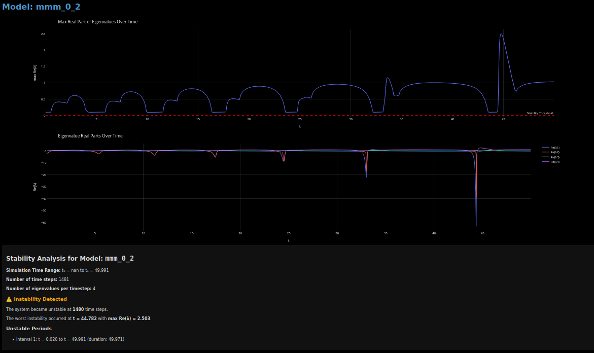
Apologies for the small fonts there. The red dashed line is the threshold, so this model is very unstable. No chance it will equilibriate. Don’t tell the Prime Minister!
In the real world, this means government will have to “meddle” and fiddle around to make domestic policy adjustments. C’mon bro! As if the Tories don’t really do that all the time.
But you’ll see at proper magnification, the maximum real eigenvalue is below 1.0 up until around $t=33.0$ time units. I think we can say that’s years since our flows are $ per year. However, supposing some sort of scale invariance, I guess with a squint of your eyes you could imagine we re-parameterized time to weeks or months. The time scale is still fairly comfy for government policy responses to avoid the cycles, if the politicians wanted to do so.
The real world political issue is they seem to never want to, and have become trained Monkeys, lassez faire is the only item on the buffet menu for our generation’s X-Gen and Boomer hold-out nasties in Parliament. So if we imagine convincing them our model is a little bit of a hint, do you think they’d reduce tax and raise spending? (Like they aught to… I mean morally so.)
Speaking of time reparameterization: in the next upgrade to mmm-0.3 we will introduce proper banking flows and some time constants, so these will be implictly dimensioned by empirical fitting. For example, you should find I introduce $\tau_P$ as a price response characteristic time, and a few other time constants. The numeric values of these parameters have to be given a unit. Although I am not using model Typing, we’ll just claim the units will be in years I think. So $\tau_P = 0.25$ is (will be) a quarterly (4-month) response time.
Hence, in this light, our silly model is only midly horrific. After 2 years we reach 46% unemployment.
I guess you might say, yeah, but that’s realistic, since in the real world 40% of all jobs are ꕗꖹꝆꝆꕷꖾꕯꖡ. And I probably would not argue. Today with U6 around 6% or whatever, we probably are at 44% unemployment effectively. (This is just an ideological remark.)
We do not have proper $\lambda$ cycles in NZ, nor anywhere in any nation I know of, since government policy variables are strnger than in our model (many automatic stabilizers), and are always being adjusted. But here’s a recent time series:
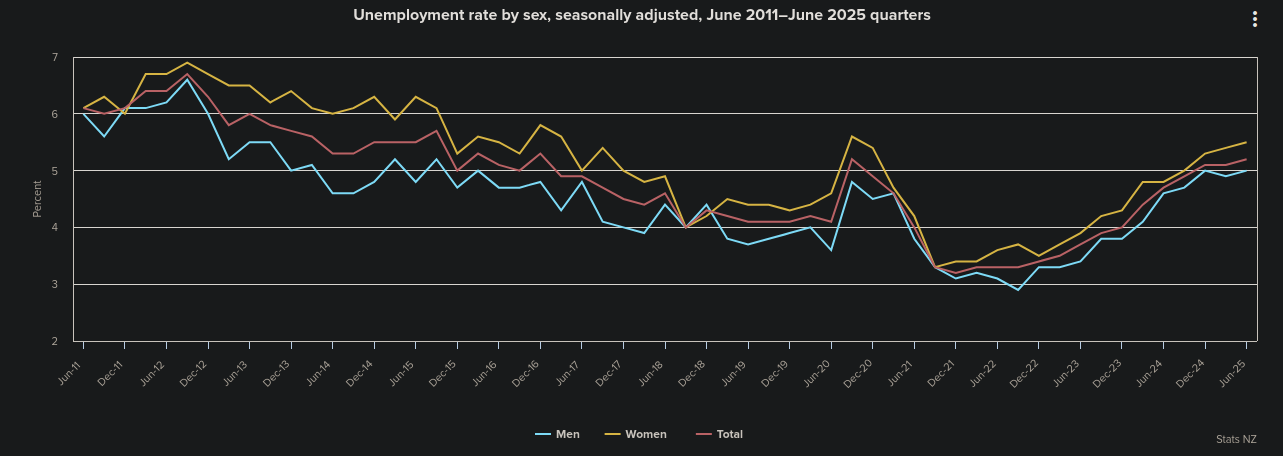
We have to stabilize our model in any case, or at least try for educational purposes.
Homework Problem
What to do? Look, I’m no expert on MMT models just yet, I don’t have that Ramanujan mystical feel for them — A Friend of the Dynamical Variables. I doubt anyone in the world is really.
Refinement–0.3
Moved this to the next chapter .
| Previous chapter | Back to | Next chapter |
| NZ ECON — 0 | TOC | MMT ODE Models — II |